Multiclass quantification#

Every quantifier in mlquantify handles more than two classes. Native multiclass methods (CC, PCC, EMQ, the KDEy family, the generalized matching methods) work on the full simplex directly. Binary methods — ACC, HDy, DyS, SORD and the threshold-selection counters — are decomposed into a set of binary sub-problems automatically, using One-vs-Rest. The diagnostics carry over either way.

Native multiclass methods#

We start with EMQ, evaluate it across many prevalence vectors with a UPP, and show a per-class diagonal plot.

from sklearn.datasets import make_classification
from sklearn.linear_model import LogisticRegression

from mlquantify.likelihood import EMQ
from mlquantify.model_selection import apply_protocol
from mlquantify.visualization import DiagonalDisplay

X, y = make_classification(
    n_samples=4500, n_features=20, n_informative=6,
    n_classes=3, n_clusters_per_class=1, random_state=0,
)

q = EMQ(LogisticRegression(max_iter=1000))
results = apply_protocol(
    q, X, y, protocol="upp",
    n_prevalences=400, batch_size=120, random_state=0,
)

# DiagonalDisplay colour-codes the three classes on one axes for multiclass.
disp = DiagonalDisplay.from_predictions(
    results["true_prevalences"], results["predicted_prevalences"],
    alpha=0.4, s=16,
)
disp.ax_.set_title("EMQ — 3-class diagonal (one colour per class)")
disp.figure_.set_size_inches(6, 6)
disp.figure_.tight_layout()

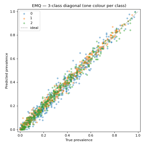
Each class gets its own colour; all three clouds hug the diagonal, confirming EMQ recovers the full prevalence vector and not just one class.

Binary methods via One-vs-Rest#

A binary quantifier cannot, by itself, estimate three prevalences. Under One-vs-Rest the problem is split into “class \(k\) vs. the rest” for every class; each sub-quantifier estimates the prevalence of its own class, and the results are normalised to sum to one. mlquantify does this transparently: you just fit and predict the binary method exactly as in the binary case — One-vs-Rest is applied automatically, since it is the default decomposition. No manual class loop, no extra configuration.

The grid below runs four binary methods on the same three-class problem.

import matplotlib.pyplot as plt
from sklearn.datasets import make_classification
from sklearn.linear_model import LogisticRegression

from mlquantify.counting import ACC
from mlquantify.matching import HDy, DyS, SORD
from mlquantify.model_selection import apply_protocol
from mlquantify.visualization import DiagonalDisplay

X, y = make_classification(
    n_samples=4500, n_features=20, n_informative=6,
    n_classes=3, n_clusters_per_class=1, random_state=0,
)

# All four are binary quantifiers — they only know "positive vs. rest".
methods = {
    "ACC": ACC(LogisticRegression(max_iter=1000)),
    "HDy": HDy(LogisticRegression(max_iter=1000)),
    "DyS": DyS(LogisticRegression(max_iter=1000)),
    "SORD": SORD(LogisticRegression(max_iter=1000)),
}

fig, axes = plt.subplots(2, 2, figsize=(9, 9))
for (name, q), ax in zip(methods.items(), axes.ravel()):
    # No manual decomposition: the binary method handles 3 classes via OvR.
    results = apply_protocol(
        q, X, y, protocol="upp",
        n_prevalences=200, batch_size=120, random_state=0,
    )
    DiagonalDisplay.from_predictions(
        results["true_prevalences"], results["predicted_prevalences"],
        ax=ax, alpha=0.4, s=14,
    )
    ax.set_title(f"{name}  (One-vs-Rest)")
fig.suptitle("Binary quantifiers on a 3-class problem via OvR", y=0.99)
fig.tight_layout()

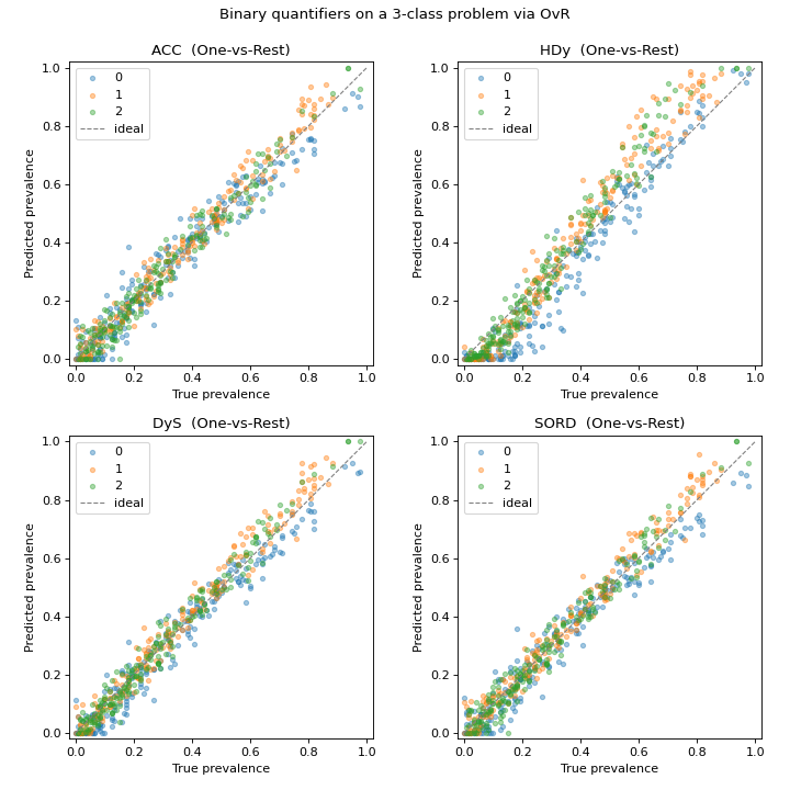
Despite being binary at heart, all four methods track the diagonal across the whole simplex: One-vs-Rest extends them to three classes with no change to your code. Each sub-quantifier estimates the prevalence of its own class, and mlquantify normalises the per-class estimates so the prediction stays a valid prevalence vector.